restrictedROC calculates restricted ROC curves, their permutation p-values, plots and multivariate random forest models with restriction.
Installation
You can install the latest version of restrictedROC like so:
devtools::install_github("ggrlab/restrictedROC")Quickstart
Given a dataset with one dependent (outcome, binary) variable and one independent (predictor, numeric) variables, e.g. the value of a biomarker in two groups of patients, we want to know if the biomarker is informative for the outcome.
set.seed(123)
biodata <- data.frame(
    outcome = factor(c(rep("Good", 50), rep("Poor", 50))),
    biomarker = c(rnorm(50, 10, 3), rnorm(50, 9, 1))
)
head(biodata)
#>   outcome biomarker
#> 1    Good  8.318573
#> 2    Good  9.309468
#> 3    Good 14.676125
#> 4    Good 10.211525
#> 5    Good 10.387863
#> 6    Good 15.145195
Here we use outcome and biomarker as dependent and independent variables, respectively. outcome is a factor with two levels, biomarker is a numeric variable.
The most convenient usage of restrictedROC is via the rROC() function. The most important results of restrictedROC::rROC() are:
- (restricted) AUCs for all possible cutoffs of the predictor variable
- A global and maximal (including all restrictions) AUC
- Permutation p-values for the global and maximal AUC
# library(restrictedROC)
set.seed(412)
res_rroc <- restrictedROC::rROC(
    x = biodata$biomarker,
    y = biodata$outcome,
    positive_label = "Good",
    n_permutations = 100 # increase that in real data!
)
#> Wed Dec  6 14:06:24 2023      y x ( 1 )
res_rroc is a nested list where the first level contains all dependent variables (Here only y). The second level contains the results for each independent variable (here only x).
Each dependent + independent variable combination has the following results:
-
plots: Plots, only if enabled, otherwise NA -
permutation: ArestrictedROCclass element containing each permutation result
single_result <- res_rroc[["y"]][["x"]][["permutation"]]Given a dataframe, you can use arbitrary dependent and independent variables (within the dataframe) and calculate the restricted ROC curve for each combination. Additionally, the list names will be set to the respective dependent (first level) and independent (second level) variable names.
set.seed(412)
res_rroc <- restrictedROC::rROC(
    x = biodata,
    dependent_vars = c("outcome"),
    independent_vars = c("biomarker"),
    positive_label = "Good",
    n_permutations = 100 # increase that in real data!
)
#> Wed Dec  6 14:06:26 2023      outcome biomarker ( 1 )
single_result <- res_rroc[["outcome"]][["biomarker"]][["permutation"]]single_result$permutation_pval refers to the permutation p-values of:
-
pval.twoside.global: The global AUC when all samples are used. This is the usually known AUC with a calculated permutation p-value. -
pval.twoside.max: This is the maximal (restricted or unrestricted) AUC’s permutation p-value.
print(round(single_result$permutation_pval, 3))
#>    pval.twoside.max pval.twoside.global      n_permutations
#>               0.010               0.069             100.000
In this particular example we see that at a significance level of 0.05, the global AUC is insignificant, but the maximal AUC is significant. This tells that the data should be restricted and has a limited informative range.
single_result$global refers to the AUC, its variance under H0, the standardized AUC, and its (asymptotic, not permutation!) p-value when using all samples without restriction.
print(single_result$global)
#>      auc auc_var_H0   rzAUC pval_asym
#> 1 0.6016     0.6016 1.75103 0.0799407
We see that the AUC is 0.6016, with a p-value of 0.08. This is not significant at a significance level of 0.05.
single_result$max_total refers to the AUC, its variance under H0, the standardized AUC, its (asymptotic, not permutation!) p-value, the threshold(=restriction value) and which part of the data is kept and therefore within the informative range.
print(single_result$max_total)
#>         auc  auc_var_H0    rzAUC    pval_asym threshold part
#> 1 0.9089069 0.007759784 4.641941 3.451517e-06  9.377944 high
In this example, the maximal AUC is 0.9089, with a restriction value of 9.377944 and a focus on the “low” part. Therefore, the informative range is biomarker < 9.378.
In particular, we observe that the AUC is much higher than the global AUC, and that the p-value is lower. This is because the data is restricted to the informative range and the AUC is calculated only on the samples with values within this range.
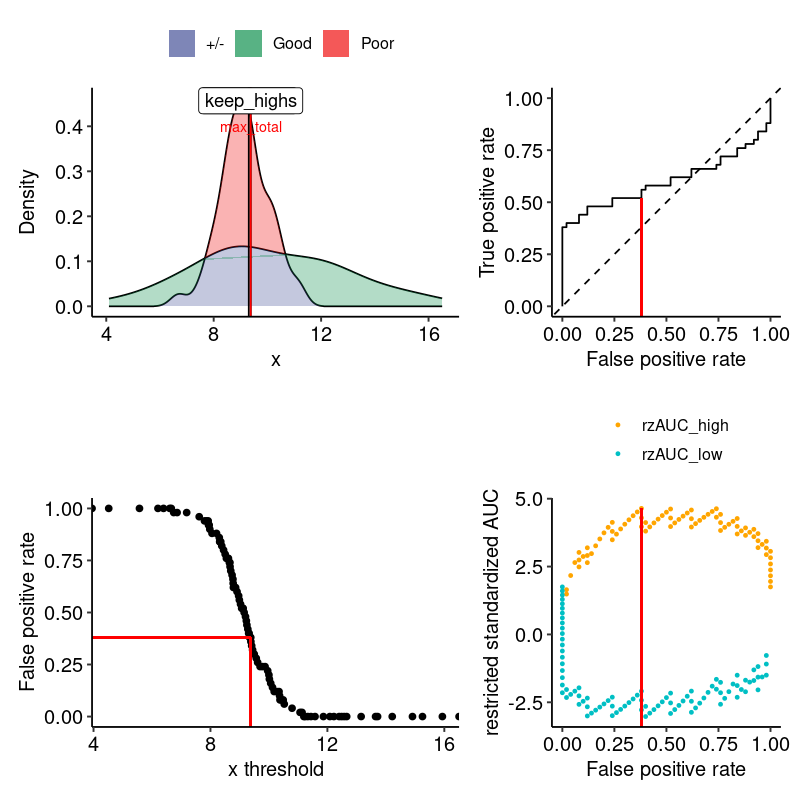
We have a convenient way to visualize the data and the results:
grouped_data <- split(biodata$biomarker, biodata$outcome)
png("man/figures/example.png", width = 800, height = 800, res = 120)
print(
    restrictedROC::plot_density_rROC_empirical(
        values_grouped = grouped_data,
        positive_label = "Good"
    )
)
#> $plots
#>
#> $single_rROC
#> $performances
#> # A tibble: 101 × 21
#>    threshold auc_high positives_high negatives_high scaling_high auc_var_H0_high
#>        <dbl>    <dbl>          <dbl>          <dbl>        <dbl>           <dbl>
#>  1   -Inf       0.602             50             50         1            0.00337
#>  2      4.52    0.614             49             50         1.02         0.00340
#>  3      5.57    0.627             48             50         1.04         0.00344
#>  4      6.20    0.64              47             50         1.06         0.00348
#>  5      6.40    0.654             46             50         1.09         0.00351
#>  6      6.61    0.668             45             50         1.11         0.00356
#>  7      6.66    0.684             44             50         1.14         0.00360
#>  8      6.74    0.677             44             49         1.16         0.00363
#>  9      6.86    0.693             43             49         1.19         0.00368
#> 10      7.19    0.709             42             49         1.21         0.00373
#> # ℹ 91 more rows
#> # ℹ 15 more variables: rzAUC_high <dbl>, pval_asym_onesided_high <dbl>,
#> #   pval_asym_high <dbl>, auc_low <dbl>, positives_low <dbl>,
#> #   negatives_low <dbl>, scaling_low <dbl>, auc_var_H0_low <dbl>,
#> #   rzAUC_low <dbl>, pval_asym_onesided_low <dbl>, pval_asym_low <dbl>,
#> #   tp <dbl>, fp <dbl>, tpr_global <dbl>, fpr_global <dbl>
#>
#> $global
#>      auc auc_var_H0   rzAUC pval_asym
#> 1 0.6016     0.6016 1.75103 0.0799407
#>
#> $keep_highs
#>         auc  auc_var_H0    rzAUC    pval_asym threshold
#> 1 0.9089069 0.007759784 4.641941 3.451517e-06  9.377944
#>
#> $keep_lows
#>         auc  auc_var_H0     rzAUC  pval_asym threshold
#> 1 0.2492063 0.006878307 -3.023958 0.00249491  9.306498
#>
#> $max_total
#>         auc  auc_var_H0    rzAUC    pval_asym threshold part
#> 1 0.9089069 0.007759784 4.641941 3.451517e-06  9.377944 high
#>
#> $positive_label
#> [1] "Good"
#>
#> $pROC_full
#>
#> Call:
#> roc.default(response = true_pred_df[["true"]], predictor = true_pred_df[["pred"]],     levels = c(FALSE, TRUE), direction = direction)
#>
#> Data: true_pred_df[["pred"]] in 50 controls (true_pred_df[["true"]] FALSE) < 50 cases (true_pred_df[["true"]] TRUE).
#> Area under the curve: 0.6016
#>
#> attr(,"class")
#> [1] "restrictedROC" "list"
dev.off()
#> png
#>   2
plot_density_rROC_empirical() effectively:
- Calls
simple_rROCto perform restriction - Makes the results readable with
simple_rROC_interpret() - Plots the original data and the restriction results